posteriors: Normal Computing’s library for Uncertainty-Aware LLMs

posteriorsis a new open source Python library from Normal Computing that provides tools for uncertainty quantification and Bayesian computation. We use PyTorch and its functional API. Online learning and hallucination detection are understood as frontier problems in AI and with LLMs. Here we introduce the posteriors library and demonstrate how it can robustify predictions and avoid catastrophic forgetting.

Uncertainty: computing the unknown 🤷

There are a number of ways which the community has begun investigating trading off compute for reliability – including adaptively – in AI models. We will discuss a path which has been less explored given scalability and accessibility questions which we seek to resolve. By investing more compute into the probabilistic inference required to perform uncertainty quantification, we can unlock LLMs that hallucinate less, understand their own limits, and even reason with higher precision.

Robust decision making needs to handle complex uncertainty. In the context of deep learning, uncertainty quantification is particularly important because neural networks are often overconfident in their predictions or generations, salmon jumping in a river anyone?

What’s more, traditional neural networks do not have the capacity to inform you when they are met with unfamiliar data or are asked about something they don’t know. By quantifying uncertainty in the model parameters, we can average predictions over many plausible model instances given the training data. This provides a compelling route to more robust predictions on unseen data. Accurate uncertainty characterisation also provides the ability to identify situations where the model is met with data beyond that it has seen in training, thus critically improving model auditability.

Bayesian updating is concisely described by Bayes’ theorem: \[ \underbrace{\; p(\theta | \mathcal{D}) \; }_\text{posterior} \propto \underbrace{\; p(\mathcal{D} | \theta) \;}_\text{likelihood} \; \underbrace{\; p(\theta) \;}_\text{prior} \]

The prior distribution encodes our current beliefs and the likelihood function relates the model parameters to the data. Bayes’ theorem then tells us exactly how to update our beliefs in the face of new data. Thus providing a cohesive framework for the continual learning of new information, which can also be used for informed online decision making.

Aren’t posterior distributions intractable? 🤯

Whilst Bayes theorem gives you a coherent way to update your beliefs in the face of new data, computing the posterior distribution is often intractable — especially when said distribution is over trillions of parameters of a neural network. The good news is that approximate posterior distributions, when computed effectively, provide many of the benefits promised by exact Bayesian inference. But they can still be tricky to deal with and hard to compute especially for Large Language Models – a massive hurdle we wanted to unlock.

Traditional techniques for Bayesian computation have typically relied on methods such as Markov chain Monte Carlo (MCMC), where the posterior distribution is represented by a set of samples (generated iteratively). MCMC methods are powerful but computationally expensive in the settings of very large datasets due to having to query all datapoints at every step of the iterative algorithm. In the context of deep learning, this can be prohibitively slow.

posteriors provides a suite of tools allowing for approximate Bayesian inference that is scalable to settings of many parameters and/or large datasets. Many of the posteriors methods have also been carefully implemented to provide a seamless transition between optimization and Bayesian computation¹.

Why posteriors? 𝞡

posteriors is designed to be a comprehensive library for uncertainty quantification in deep learning models. The key features outlining the posteriors philosophy are:

• PyTorch: posteriors is built on top of PyTorch, this means that it can be integrated with pre-trained models such as Llama2 and Mistral via Hugging Face’s transformers package. posteriors takes elements of the JAX packages fortuna and blackjax (plus more) and brings them to the PyTorch ecosystem.
• Functional: posteriors adopts a functional API via torch.func. The functional approach, as championed by the JAX ecosystem, makes for code that is easier to test and compose with other functions. Importantly for posteriors, functional programming is also closer to the mathematical description which is particularly useful for Bayesian modelling.
• Extensible: The transform framework² adopted by posteriors is very general and allows for the easy adoption of new algorithms. Additionally, posteriors supports arbitrary likelihoods³ rather than being restricted to hard coded regression or classification as is common in other libraries like fortuna or laplace.
• Swappable: The framework also allows the user to seamlessly switch between approaches.
• Scalable: posteriors is minibatch first thus allowing for efficient computation in large datasets. Additionally flexible subspace methods are provided for scaling to large models.
• Composable: posteriors composes seamlessly with other torch libraries including transformers for pre-trained models, torch.distributions for probabilistic modeling, torchopt for functional optimization and lightning for convenient logging and training.

The python ecosystem is rich with wonderful tools for deep learning and uncertainty. Including fortuna, laplace, blackjax, numpyro, uncertainty-baselines and more, however none meet all of the above criteria. posteriors is designed to be a one-stop shop for uncertainty quantification in deep learning models.

posteriors is open-source! Come try it out, raise an issue or contribute a method! github.com/normal-computing/posteriors

Learning without forgetting 🔄

The key difficulty in continual learning is adapting to new data without forgetting what has been learned before, so-called catastrophic forgetting. In our continual_lora example we demonstrate how a Laplace approximation using posteriors can be used to help Llama-2-7b retain old information whilst it is trained on a series of books from the pg19 dataset.

Figure 1: Continual validation loss by episode

 

Figure 2: Average cumulative validation performance

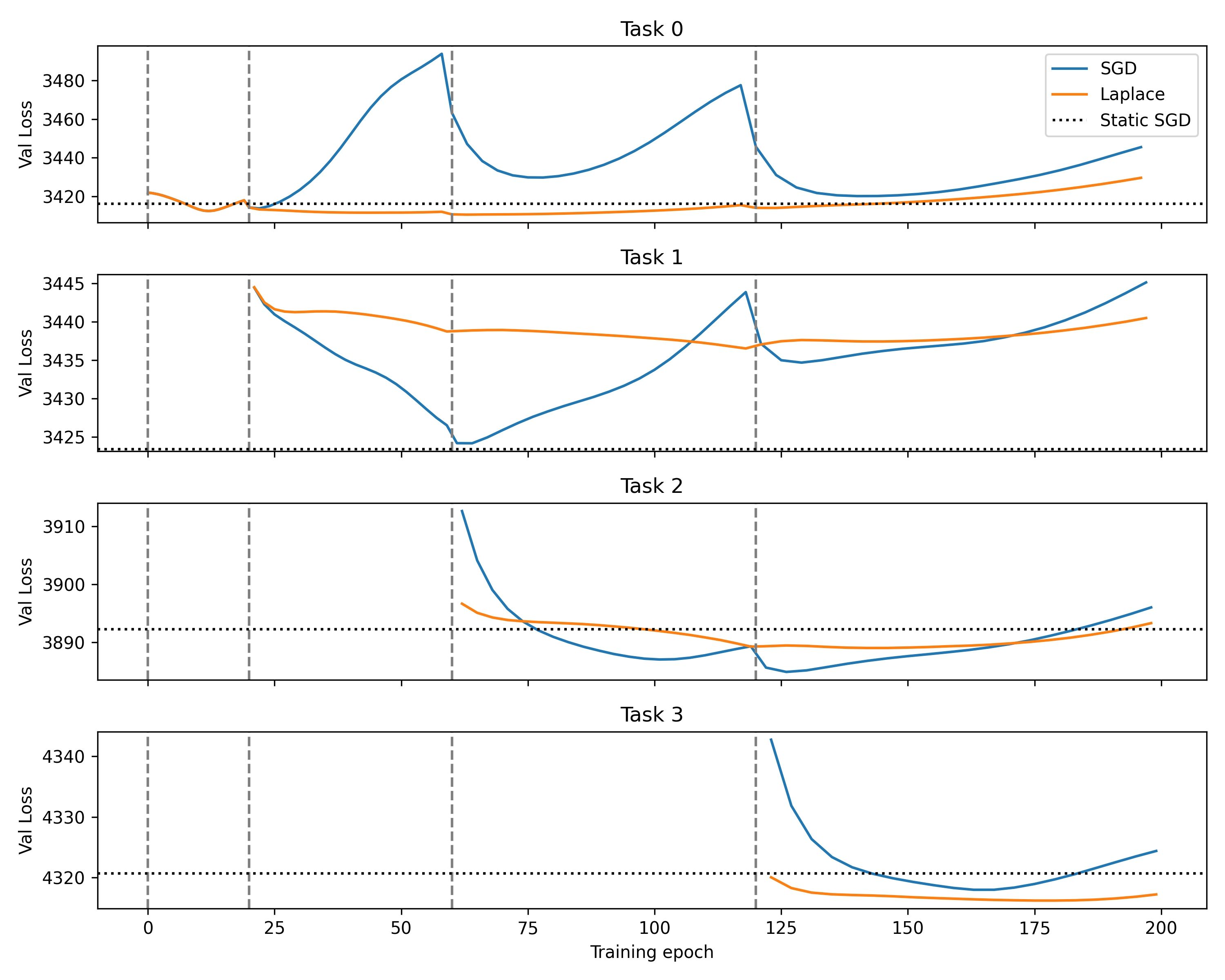
In Figure 1, we compare the continual learning of the LLM stochastic gradient descent (AdamW) against a Bayesian inspired Laplace approximation approach. The dashed vertical lines represents “new episodes” where the model starts training on a new book - after this point the model does not see the book again. The horizontal dashed lines represent a single offline train with access to all four training datasets concurrently; the network’s total learning capacity, although this isn’t feasible in a practical online setting. Each row represents validation loss for a different book. For example, in the first row we can see that the SGD approach quickly forgets the information it has learned from the first book as it trains on new books, whereas the Bayesian LLM encourages the model to retain knowledge.

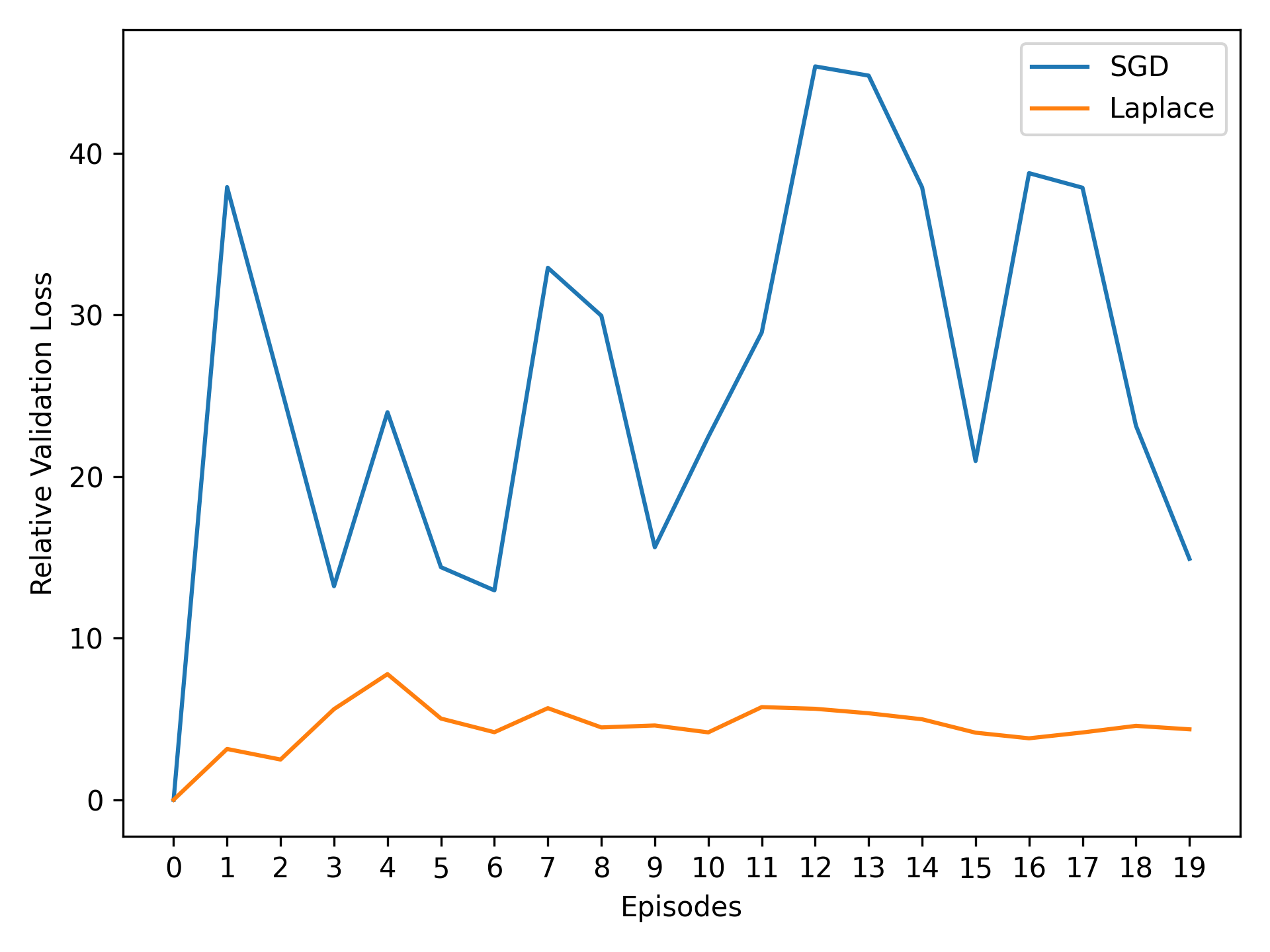
In Figure 2, we track the average performance⁴ of the two approaches over books seen so far. We can see that SGD, when averaged across all tasks performs extremely⁵ poorly compared to the Bayesian LLM. The key thing here is that the use of the approximate Bayesian method allows you to use a single model to learn across multiple tasks whereas with traditional methods you would need to train a new model for each task.

This example demonstrates how posteriors can be used to implement a continual learning strategy and assist the model in learning tasks sequentially. However, the Laplace approximation represents a very simple and somewhat crude approximation to Bayesian updating, certainly there is room for further improvement. posteriors can help with this! Via its flexible and extensible framework we can add and compare different and new approaches.

Further information on this example (and others) including complete code can be found on GitHub.

Knowing what you don’t know 🤔

Bayesian methods provide the ability to break predictive uncertainty into two components: aleatoric and epistemic uncertainty⁶. Aleatoric uncertainty is the uncertainty inherent in the data itself (for example, a review like “The food was amazing! But the service was horrendous!” would have a high amount of aleatoric uncertainty when predicting the associated rating), whereas epistemic uncertainty would be reduced with more data. High epistemic uncertainty is an indication that the model is unsure about the data it is being asked to predict.

So in principle, we might hope to use epistemic uncertainty as a measure to predict hallucinations in LLMs – low confidence should correlate with mistakes.

Figure 3: Uncertainty breakdown on English test data (in-distribution).

 

Figure 4: Uncertainty breakdown on Spanish test data (out-of-distribution).

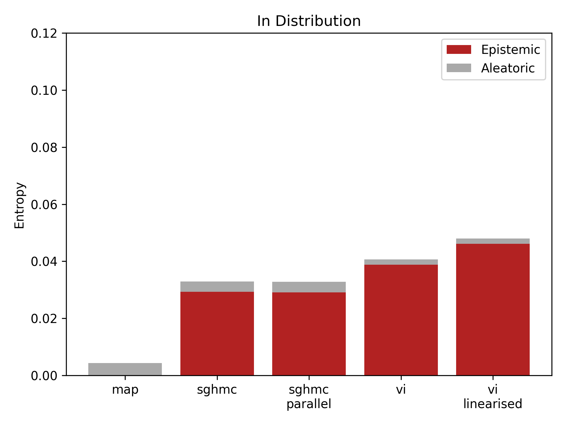
In the yelp example, we use posteriors to train a host of Bayesian methods on the Yelp review dataset (English). In Figure 3, we show the breakdown of uncertainty on the in-distribution English data. We compare this to uncertainty on out-of-distribution Spanish data in Figure 4. The non-Bayesian optimisation (map) method does not provide the ability to breakdown uncertainty, whereas the Bayesian methods successfully identify an increase in epistemic uncertainty on the out-of-distribution data, allowing us to infer that the model does not know the answer in this case and would like to have some Spanish training data to make more accurate predictions.

As before, comprehensive code and info on GitHub!

What’s next? 🔜

posteriors is a new Python library designed to make it possible to apply uncertainty quantification to large-scale deep learning models. This represents a key component of Normal Computing’s mission to build AI systems that natively reason, so they can partner with us on our most important problems. We are excited to expand posteriors and support community efforts to improve the auditability and robustness of AI systems, as well as integrating with thermodynamic compute that can accelerate Bayesian posteriors methods. If you are as interested as we are in advancing the frontier of AI reasoning and reliability then reach out to us at [email protected]!

Footnotes

1. Typically through a temperature parameter where temperature=0 represents optimisation and temperature=1 represents Bayes. With values in between also valid.

2. posteriors conforms to a very general unified API where each method is comprised of build, init and update functions.

3. There is an equivalence between the negative-log-likelihood function and the loss function in the context of maximum likelihood estimation. For example, a likelihood with a conditional Gaussian distribution is the same as the mean squared error loss function for regression and conditional Categorial distribution is the same as cross entropy for classification.

4. To be exact, relative to the perfomance of the model trained to convergence on each individual book

5. catastrophically, perhaps?

6. Further details on second-order uncertainty can be found in e.g. Wimmer et al. It should be noted that the entropy approach to breaking down uncertainty has some potentially undesirable features and, in the Bayesian setting, can be sensitive to inaccuracies in the posterior approximation.